Analyzing Hass USA

The {avocado} package provides a weekly summary - starting from January 2017 through November 2020 - of Hass Avocado sales. There are three datasets in this package and let’s start with the dataset hass_usa which focuses on weekly avocado sales in the contiguous US.

Let’s start by loading the package - along with {dplyr} (for data wrangling) and {ggplot} (for data visualization) - and exploring it’s structure

library(avocado)
library(dplyr)
#> 
#> Attaching package: 'dplyr'
#> The following objects are masked from 'package:stats':
#> 
#>     filter, lag
#> The following objects are masked from 'package:base':
#> 
#>     intersect, setdiff, setequal, union
library(ggplot2)

data('hass_usa')

dplyr::glimpse(hass_usa)
#> Rows: 197
#> Columns: 15
#> $ week_ending       <dttm> 2017-01-02, 2017-01-08, 2017-01-15, 2017-01-22, 20…
#> $ avg_price_nonorg  <dbl> 0.89, 0.99, 0.98, 0.94, 0.96, 0.77, 0.87, 0.99, 0.9…
#> $ plu4046           <dbl> 12707895, 11809728, 12936858, 14254150, 14034076, 2…
#> $ plu4225           <dbl> 14201201, 13856935, 12625665, 14212882, 11683465, 2…
#> $ plu4770           <dbl> 549844.6, 539068.4, 579346.5, 908616.4, 818727.0, 1…
#> $ small_nonorg_bag  <dbl> 8551134, 9332972, 9445622, 9462854, 9918256, 125671…
#> $ large_nonorg_bag  <dbl> 2802709, 2432259, 2638918, 3231020, 2799961, 361827…
#> $ xlarge_nonorg_bag <dbl> 66933.73, 78840.96, 69077.52, 70871.48, 119095.66, …
#> $ avg_price_org     <dbl> 1.48, 1.43, 1.44, 1.37, 1.43, 1.36, 1.41, 1.31, 1.2…
#> $ plu94046          <dbl> 99820.77, 117721.87, 121132.79, 115700.02, 131808.2…
#> $ plu94225          <dbl> 273329.61, 283532.68, 280287.84, 281786.33, 292584.…
#> $ plu94770          <dbl> 4425.75, 8697.35, 8750.08, 6707.82, 3524.96, 2238.7…
#> $ small_org_bag     <dbl> 273456.00, 379088.19, 400292.46, 401805.90, 346391.…
#> $ large_org_bag     <dbl> 157939.75, 201681.74, 165261.11, 188282.91, 178896.…
#> $ xlarge_org_bag    <dbl> 0, 0, 0, 0, 0, 0, 0, 0, 0, 0, 0, 0, 0, 0, 0, 0, 0, …

Exploratory Data Analysis

Let’s begin by exploring the following two topics:

• Fluctuation of average selling price
• Non Organic Avocado sales revenue

Fluctuation of Average Selling Price

hass_usa %>%
  ggplot(aes(x = week_ending)) +
  geom_line(aes(y = avg_price_nonorg, color = 'Non Organic')) +
  geom_line(aes(y = avg_price_org, color = 'Organic')) +
  scale_color_manual(values = c('steelblue','forestgreen')) +
  labs(x = 'Year', y = 'Average Price per Pound in US$', color = 'Type', title = 'Average Selling Price by Week', caption = 'Not adjusted for inflation\nSource: Hass Avocado Board') +
  ylim(min = 0, max = 3.0) +
  theme(plot.background = element_rect(fill = "grey20"),
        plot.title = element_text(color = "#FFFFFF"),
        axis.title = element_text(color = "#FFFFFF"),
        axis.text.x = element_text(color = 'grey50', angle = 45, hjust = 1),
        axis.text.y = element_text(color = 'grey50'),
        plot.caption = element_text(color = 'grey75'),
        panel.background = element_blank(),
        panel.grid.major = element_line(color = "grey50", size = 0.2),
        panel.grid.minor = element_line(color = "grey50", size = 0.2),
        legend.background = element_rect(fill = 'grey20'),
        legend.key = element_rect(fill = 'grey20'),
        legend.title = element_text(color = 'grey75'),
        legend.text = element_text(color = 'grey75'),
        legend.position = c(0.815, 0.85)
        )

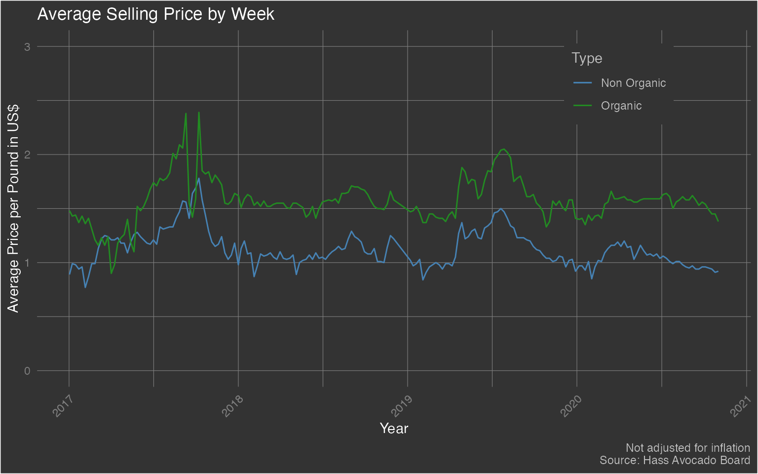
Unsurprisingly, we can see that the average selling price for organic avocados tends to be higher than the average selling price for non-organic avocados. Note how there seems to be a fairly large spike in selling price in late 2017.

Non Organic Avocado Sales Revenue

hass_usa %>%
  mutate(
    nonorg_rev = (plu4046+plu4225+plu4770+small_nonorg_bag+large_nonorg_bag+xlarge_nonorg_bag) * avg_price_nonorg
  ) %>%
  ggplot(aes(x = week_ending)) +
  geom_line(aes(y = nonorg_rev/1000000), color = 'steelblue') +
  labs(x = 'Year', y = 'Revenue (Millions US$)', color = 'Type', title = 'Non Organic Avocado Sales Revenue', caption = 'Not adjusted for inflation\nSource: Hass Avocado Board') +
  theme(plot.background = element_rect(fill = "grey20"),
        plot.title = element_text(color = "#FFFFFF"),
        axis.title = element_text(color = "#FFFFFF"),
        axis.text.x = element_text(color = 'grey50'),
        axis.text.y = element_text(color = 'grey50'),
        plot.caption = element_text(color = 'grey75'),
        panel.background = element_blank(),
        panel.grid.major = element_line(color = "grey50", size = 0.2),
        panel.grid.minor = element_line(color = "grey50", size = 0.2),
        legend.background = element_rect(fill = 'grey20'),
        legend.key = element_rect(fill = 'grey20'),
        legend.title = element_text(color = 'grey75'),
        legend.text = element_text(color = 'grey75'),
        # legend.position = c(0.815, 0.2)
        legend.position = 'none'
  )

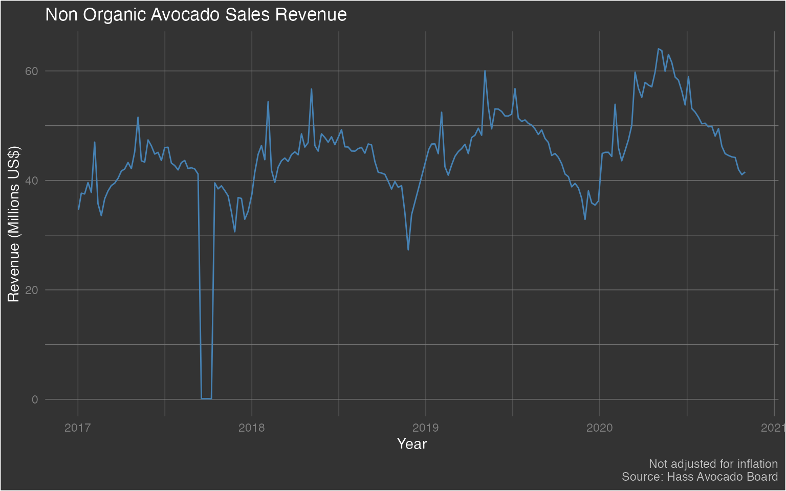
We may have switched gears from looking at average selling price to revenue. However, notice the massive drop in revenue in late 2017 - which seems to correspond to the increase in average selling price for the same time period.

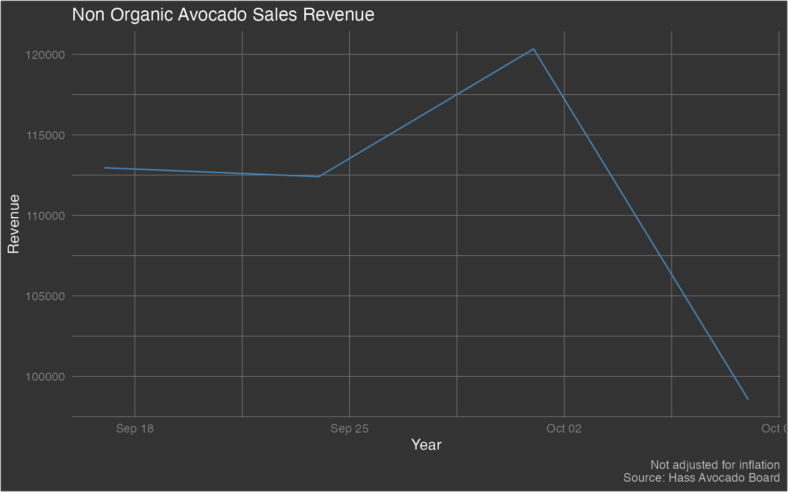
Let’s dive further into that ‘dip’.

hass_usa %>%
  mutate(
    nonorg_rev = (plu4046+plu4225+plu4770+small_nonorg_bag+large_nonorg_bag+xlarge_nonorg_bag) * avg_price_nonorg
  ) %>%
  select(week_ending, nonorg_rev) %>%
  filter(week_ending > lubridate::ymd('2017-09-10') & week_ending < lubridate::ymd('2017-10-15')) %>%
  ggplot(aes(x = week_ending, y = nonorg_rev)) +
  geom_line(color = 'steelblue') +
  labs(x = 'Year', y = 'Revenue', color = 'Type', title = 'Non Organic Avocado Sales Revenue', caption = 'Not adjusted for inflation\nSource: Hass Avocado Board') +
  theme(plot.background = element_rect(fill = "grey20"),
    plot.title = element_text(color = "#FFFFFF"),
    axis.title = element_text(color = "#FFFFFF"),
    axis.text.x = element_text(color = 'grey50'),
    axis.text.y = element_text(color = 'grey50'),
    plot.caption = element_text(color = 'grey75'),
    panel.background = element_blank(),
    panel.grid.major = element_line(color = "grey50", size = 0.2),
    panel.grid.minor = element_line(color = "grey50", size = 0.2),
    legend.background = element_rect(fill = 'grey20'),
    legend.key = element_rect(fill = 'grey20'),
    legend.title = element_text(color = 'grey75'),
    legend.text = element_text(color = 'grey75'),
    legend.position = 'none'
  )

So we can see that the revenue wasn’t exactly 0. However, it definitely was much lower (way less than a US$1 million). A quick search on the Internet shows that around that time frame, there was a major avocado supply shortage in the US.